Switching from Legacy Software

This section provides basic switcher’s guide for those who are familar with ASTROLIB PYSYNPHOT or IRAF SYNPHOT. It complements the switcher’s guide for synphot that covers the more general functionalities. This guide is not meant to be all-inclusive; Therefore, not all legacy commands are listed here. This is because a legacy command can be reproduced in several different ways using stsynphot or has no equivalent implementation. Naming convention used is the same as Quick Guide. Please contact STScI Help Desk if you have any questions.

ASTROLIB Switcher Guide

Bandpass

stsynphot	ASTROLIB PYSYNPHOT
band(obsmode)	ObsBandpass(obsmode)
bp.binset	bp.binset
bp.area	bp.primary_area
len(bp)	len(bp)
bp.showfiles()	bp.showfiles()
bp.thermback()	bp.thermback()

Other Spectrum

stsynphot	ASTROLIB PYSYNPHOT
ebmvx(law, val)	Extinction(val, law)
Vega	Vega
grid_to_spec(model, Teff, Z, log_g)	Icat(model, Teff, Z, log_g)
parse_spec(iraf_string)	parse_spec(iraf_string)

Configuration

stsynphot	ASTROLIB PYSYNPHOT
showref()	showref()
getref()	getref()
conf.reload() # From stsynphot.cfg conf.reset() # Hardcoded default	setref()
conf.graphtable = ‘mytmg.fits’	setref(graphtable=’mytmg.fits’)
conf.comptable = ‘mytmc.fits’	setref(comptable=’mytmc.fits’)
conf.thermtable = ‘mytmt.fits’	setref(thermtable=’mytmt.fits’)
conf.area = 123.4	setref(area=123.4)
conf.waveset_array = numpy.logspace( 1, 4, 1000, endpoint=False) conf.waveset = ‘Min: 10, Max: 10000, Num: 1000, Delta: None, Log: True’	setref(waveset=(10, 10000, 1000))
conf.waveset_array = numpy.linspace( 10, 10000, 1000, endpoint=False) conf.waveset = ‘Min: 10, Max: 10000, Num: 1000, Delta: None, Log: False’	setref(waveset=(10, 10000, 1000, ‘linear’))

IRAF Switcher Guide

Bandpass

sysynphot	IRAF SYNPHOT
band(obsmode)	band(obsmode)
bp.area	refdata.area
bp.showfiles()	showfiles obsmode
bp.thermback()	thermback obsmode

Other Spectrum

stsynphot	IRAF SYNPHOT
ebmvx(law, val)	ebmvx(val, law)
grid_to_spec(model, Teff, Z, log_g)	icat(model, Teff, Z, log_g)
parse_spec(iraf_string)	See IRAF Language Parser

Configuration

stsynphot	IRAF SYNPHOT
showref()	lpar refdata
conf.reload() # From stsynphot.cfg conf.reset() # Hardcoded default	unlearn refdata
conf.graphtable = ‘mytmg.fits’ conf.comptable = ‘mytmc.fits’ conf.area = 123.4	epar refdata

Examples

The examples below show how to accomplish some real use cases in both IRAF SYNPHOT and stsynphot. The IRAF commands are preceded by sy>; They are followed by the Python equivalent in >>>. Some examples were adapted from old IRAF SYNPHOT documentation; Therefore, any differences between the results could be due to the fact that CRDS data have changed over time.

IRAF setup:

iraf> stsdas
iraf> hst_calib
iraf> synphot
sy>

Python imports:

>>> import os
>>> import stsynphot as stsyn
>>> from synphot import units, SourceSpectrum, Observation
>>> from synphot.models import BlackBodyNorm1D

Calculate the pivot wavelength, the equivalent Gaussian FWHM, and the total flux (in counts/s) of a 5000 K blackbody in the HST/WFPC F555W bandpass. The blackbody spectrum is normalized to be 18.6 VEGAMAG in V-band:

sy> calcphot "band(wfpc,f555w)" "rn(bb(5000),band(v),18.6,vegamag)" counts
Mode = band(wfpc,f555w)
Pivot       Equiv Gaussian
Wavelength  FWHM
5467.653    1200.953    band(wfpc,f555w)
Spectrum:  rn(bb(5000),band(v),18.6,vegamag)
VZERO      (COUNTS s^-1 hstarea^-1)
0.           419.5938

>>> rnbb = SourceSpectrum(BlackBodyNorm1D, temperature=5000).normalize(
...     18.6 * units.VEGAMAG, band=stsyn.band('v'), vegaspec=stsyn.Vega)
>>> obs = Observation(rnbb, stsyn.band('wfpc,f555w'))
>>> print(f'Pivot Wavelength: {obs.bandpass.pivot():.3f}\n'
...       f'Equiv Gaussian FWHM: {obs.bandpass.fwhm():.3f}\n'
...       f'Countrate: {obs.countrate(stsyn.conf.area):.4f}')
Pivot Wavelength: 5467.651 Angstrom
Equiv Gaussian FWHM: 1200.923 Angstrom
Countrate: 416.4439 ct / s

Calculate the total flux (in OBMAG) of a 5000 K blackbody in the HST/ACS WFC1 F555W bandpass for \(E(B-V)\) values of 0.0, 0.25, and 0.5:

sy> calcphot "acs,wfc1,f555w" "bb(5000)*ebmv($0)" obmag vzero="0.0,0.25,0.5"
Mode = band(acs,wfc1,f555w)
Pivot       Equiv Gaussian
Wavelength  FWHM
5361.008    847.9977    band(acs,wfc1,f555w)
Spectrum:  bb(5000)*ebmv($0)
VZERO      (OBMAG s^-1 hstarea^-1)
0.           -10.0087
0.25         -9.1981
0.5          -8.39187

>>> law = 'mwavg'  # stsynphot has no obsolete ebmv(), so use this instead
>>> sp = SourceSpectrum(BlackBodyNorm1D, temperature=5000)
>>> bp = stsyn.band('acs,wfc1,f555w')
>>> for ebv in (0.0, 0.25, 0.5):
...     if ebv == 0:
...         print('VZERO\tOBMAG')  # Header
...     obs = Observation(sp * stsyn.ebmvx(law, ebv), bp)
...     print(f'{ebv}\t{obs.effstim(units.OBMAG, area=stsyn.conf.area):.4f}')
VZERO   OBMAG
0.0     -10.0118 OBMAG
0.25    -9.2167 OBMAG
0.5     -8.4256 OBMAG

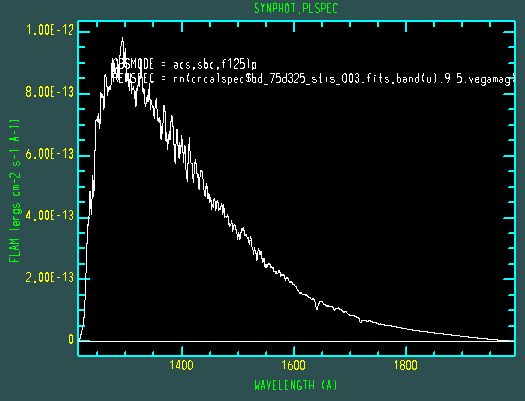
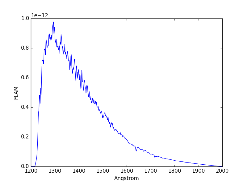
Plot an observation of BD+75 325 using the HST/ACS SBC F125LP bandpass in the unit of FLAM. The spectral data for BD+75 325 are stored in $PYSYN_CDBS/calspec/bd_75d325_stis_003.fits file. Because this spectrum has been arbitrarily normalized in intensity, we must first renormalize it to its proper magnitude of 9.5 VEGAMAG in U-band:

sy> plspec "acs,sbc,f125lp" "rn(crcalspec$bd_75d325_stis_003.fits,band(u),9.5,vegamag)" flam

>>> filename = os.path.join(
...     os.environ['PYSYN_CDBS'], 'calspec', 'bd_75d325_stis_003.fits')
>>> sp = SourceSpectrum.from_file(filename).normalize(
...     9.5 * units.VEGAMAG, band=stsyn.band('u'), vegaspec=stsyn.Vega)
>>> obs = Observation(sp, stsyn.band('acs,sbc,f125lp'))
>>> obs.plot(flux_unit=units.FLAM, left=1200, right=2000)

IRAF Language Parser

Like ASTROLIB PYSYNPHOT, stsynphot also has a special parser (parse_spec()) that can read some of the legacy IRAF SYNPHOT language for spectrum objects. The parser is based on SPARK 0.6.1 by John Aycock, which utilizes the Earley parser (Earley 1968, page 27; Earley 1970). The language is described in Laidler et al. (2005). For legacy commands that are not supported by the parser (e.g., calcphot and bandpar), please refer to IRAF Switcher Guide for alternatives.

The following table lists the available operations:

Parser Syntax	stsynphot Equivalent
band(obsmode)	band(obsmode)
bb(teff)	SourceSpectrum(BlackBodyNorm1D, temperature=teff)
box(mu, width)	SpectralElement(Box1D, amplitude=1, x_0=mu, width=width)
ebmvx(val, law)	ebmvx(law, val)
em(mu, fwhm, flux, form)	SourceSpectrum(GaussianFlux1D, mean=mu, fwhm=fwhm, total_flux=flux*form)
icat(model, Teff, Z, log_g)	grid_to_spec(model, Teff, Z, log_g)
pl(refval, expon, form)	SourceSpectrum(PowerLawFlux1D, amplitude=1*form, x_0=refval, alpha=expon)
rn(sp, bp, val, form)	sp.normalize(val*form, band=bp)
spec(filename)	SourceSpectrum.from_file(filename)
unit(val, form)	SourceSpectrum(ConstFlux1D, amplitude=val*form)
z(sp, z)	SourceSpectrum(sp.model, z=z)

These are the flux units (form) recognized by the parser (for wavelength, only Angstrom is accepted):

• abmag

• counts

• flam

• fnu

• jy

• mjy

• obmag

• photlam

• photnu

• stmag

• vegamag

These are the reddening laws (law) recognized by the parser for the ebmvx command above:

• gal3 (same as mwavg)

• lmc30dor

• lmcavg

• mwavg

• mwdense

• mwrv21

• mwrv40

• smcbar

• xgalsb

This example shows how a blackbody can be generated using both the parser and the Pythonic command. It also shows that they are equivalent:

>>> import stsynphot as stsyn
>>> from synphot import SourceSpectrum
>>> from synphot.models import BlackBodyNorm1D
>>> from numpy.testing import assert_allclose
>>> bb1 = stsyn.parse_spec('bb(5000)')
>>> bb2 = SourceSpectrum(BlackBodyNorm1D, temperature=5000)
>>> assert_allclose(bb1.integrate(), bb2.integrate())

Meanwhile, this example shows how to use the parser to apply extinction to a redshifted and renormalized spectrum obtained from a catalog. It also generates the same spectrum using Pythonic commands and compares them. Even though the Pythonic way takes more lines of codes to accomplish, one might also argue that it is more readable:

>>> from astropy import units as u
>>> sp1 = stsyn.parse_spec(
...     'ebmvx(0.1, lmcavg) * z(rn(icat(k93models, 5000, -0.5, 4.4), '
...     'band(johnson,v), 18, abmag), 0.01)')
>>> rnsp = stsyn.grid_to_spec('k93models', 5000, -0.5, 4.4).normalize(
...     18 * u.ABmag, band=stsyn.band('johnson,v'))
>>> rnsp.z = 0.01
>>> sp2 = stsyn.ebmvx('lmcavg', 0.1) * rnsp
>>> assert_allclose(sp1.integrate(), sp2.integrate())