Source Spectrum
In addition to
source spectrum in synphot, stsynphot
adds the capability to use CRDS Database for creating sources
from Catalogs and Spectral Atlases. The spectrum module also provides
the following for convenience, especially for those who are used to having them
available in ASTROLIB PYSYNPHOT:
ebmvx(), which shortens the two-step creation of an extinction curve from a reddening law into one. In addition, it also acceptsNoneand'gal3'as a reddening law to be backward compatible. For performance, any loaded reddening law is cached, which can be cleared usingreset_cache().stsynphot.spectrum.Vega, which is a preloaded Vega spectrum. It can be reloaded usingload_vega()if necessary.
Special note on count rate:
When countrate() is used for a HST
observation (also see
observation in synphot), it has two unique
features below that are ideally suited for predicting exposure times
(e.g., using HST ETC) when writing HST proposals:
The input parameters were originally structured to mimic what is contained in the exposure logsheets found in HST observing proposals in Astronomer’s Proposal Tool (APT).
For the spectroscopic instruments, it will automatically search for and use a wavelength binning that is appropriate for the selected instrumental dispersion mode.
Catalogs and Spectral Atlases
There are many spectral atlases consisting of both observed and model data that are available for use with stsynphot. For these spectra, renormalization is often necessary as they had been arbitrarily normalized before.
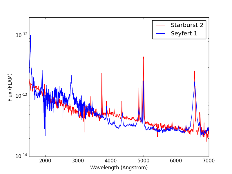
Plotting the spectra is a handy way to explore the contents. For instance, if you are interested in making some HST observations of Seyfert galaxies and want to see what sort of template spectra are available to be used with stsynphot to predict observed count rates, a good place to look would be in AGN Atlas or Kinney-Calzetti Atlas. The example below plots the spectra of a starburst and a Seyfert 1 galaxies from their respective atlases:
>>> import os
>>> import matplotlib.pyplot as plt
>>> from synphot import SourceSpectrum
>>> starburst = SourceSpectrum.from_file(os.path.join(
...     os.environ['PYSYN_CDBS'], 'grid', 'kc96', 'starb2_template.fits'))
>>> seyfert1 = SourceSpectrum.from_file(os.path.join(
...     os.environ['PYSYN_CDBS'], 'grid', 'agn', 'seyfert1_template.fits'))
>>> wave = range(1500, 7000)
>>> plt.semilogy(wave, starburst(wave, flux_unit='flam'), 'r',
...              wave, seyfert1(wave, flux_unit='flam'), 'b')
>>> plt.xlim(1500, 7000)
>>> plt.ylim(1E-14, 2E-12)
>>> plt.xlabel('Wavelength (Angstrom)')
>>> plt.ylabel('Flux (FLAM)')
>>> plt.legend(['Starburst 2', 'Seyfert 1'], loc='upper right')

For most of the catalogs and atlases (except the three mentioned below), you can load a spectrum from file once you have identified the desired filename that corresponds to the spectral parameters that you want, as shown in the example above.
However, three of the atlases (Castelli-Kurucz Atlas,
Kurucz Atlas, and Phoenix Models)
have a grid of basis spectra which are indexed for various combinations of
effective temperature (\(T_{\text{eff}}\)) in Kelvin, metallicity
([M/H]), and log surface gravity (\(\log g\)). They are best
accessed with a grid_to_spec().
You may specify any combination of the properties, so long as each is
within the allowed range, which differs from atlas to atlas. For example,
Castelli-Kurucz Atlas allows
\(3500 \; \text{K} \le T_{\text{eff}} \le 50000 \; \text{K}\),
which means that no spectrum can be constructed for effective temperatures
below 3499 K or above 50001 K (i.e., an exception will be raised).
The example below obtains the spectrum for a
Kurucz Atlas model with
\(T_{\text{eff}} = 6000 \; \text{K}\), [M/H] = 0, and
\(\log g = 4.3\):
>>> import stsynphot as stsyn
>>> sp = stsyn.grid_to_spec('k93models', 6440, 0, 4.3)
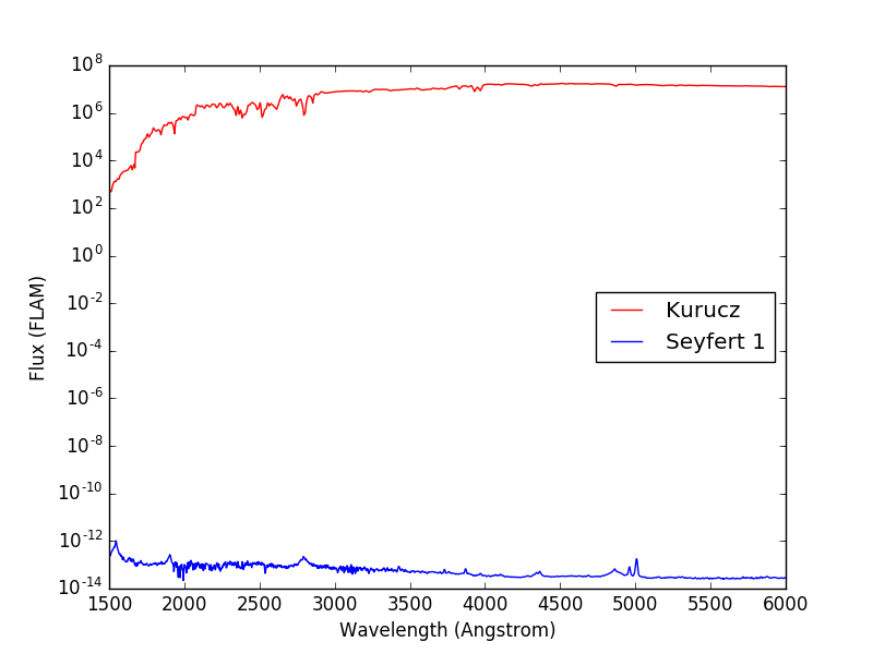
For completeness, the Kurucz spectrum is plotted below in comparison with
the Seyfert 1 from above. Note that the Kurucz spectrum has arbitrary
flux values and would need to be renormalize using
normalize() (not done here):
>>> plt.semilogy(wave, sp(wave, flux_unit='flam'), 'r',
...              wave, seyfert1(wave, flux_unit='flam'), 'b')
>>> plt.xlim(1500, 6000)
>>> plt.xlabel('Wavelength (Angstrom)')
>>> plt.ylabel('Flux (FLAM)')
>>> plt.legend(['Kurucz', 'Seyfert 1'], loc='center right')

For performance, the grid data is cached. You can use
reset_cache() to clear the cache.
