Synthetic Photometry for HST (stsynphot)
Introduction
stsynphot is an extension to synphot (Lim et al. 2016) that implements synthetic photometry package for HST support. The documentation in this package is meant to complement that of synphot, which already documents the non-observatory specific functionalities. It is recommended that you read both for full understanding of its capabilities.
This package, in particular, allows you to:
Construct spectra from various grids of model atmosphere spectra, parameterized spectrum models, and atlases of stellar spectrophotometry.
Simulate observations specific to HST.
Compute photometric calibration parameters for any supported instrument mode.
Plot instrument-specific sensitivity curves and calibration target spectra.
Like ASTROLIB PYSYNPHOT (Lim et al. 2015), stsynphot can help HST observers to perform cross-instrument simulations and examine the transmission curve of the Optical Telescope Assembly (OTA) and spectra of calibration targets.
If you use stsynphot in your work, please cite it as, CITATION for details on how to cite it in your publications.
If you have questions or concerns regarding the software, please open an issue at https://github.com/spacetelescope/stsynphot_refactor/issues (if not already reported) or contact STScI Help Desk.
Installation and Setup
stsynphot works for Python 3.11 or later only. It requires the following packages:
numpy
astropy
scipy
synphot
beautifulsoup4
matplotlib (optional for plotting)
You can install stsynphot using one of the following ways:
From the
conda-forgechannel:conda install stsynphot -c conda-forge
From standalone release on PyPI:
pip install stsynphot
From source (example shown is for the
devversion):git clone https://github.com/spacetelescope/stsynphot_refactor.git cd stsynphot_refactor pip install -e .
As with ASTROLIB PYSYNPHOT, the data files for stsynphot are distributed
separately by
Calibration Reference Data System.
They are expected to follow a certain directory structure under the root
directory, identified by the PYSYN_CDBS environment variable that must be
set prior to using this package. In the examples below, the root directory is
arbitrarily named /my/local/dir/trds.
In bash shell:
export PYSYN_CDBS=/my/local/dir/trds
In csh shell:
setenv PYSYN_CDBS /my/local/dir/trds
Below are the instructions to install:
To ensure consistency for all data files used, stsynphot silently overwrites synphot data file locations within the Python session. For example:
>>> from synphot.config import conf as syn_conf
>>> print(syn_conf.johnson_v_file)
https://ssb.stsci.edu/trds/comp/nonhst/johnson_v_004_syn.fits
>>> from stsynphot.config import conf
>>> print(conf.rootdir)
/my/local/dir/trds
>>> print(syn_conf.johnson_v_file)
/my/local/dir/trds/comp/nonhst/johnson_v_004_syn.fits
You can also take advantage of
Astropy configuration system to manage
stsynphot configuration and data files. For example, with astropy,
you can generate a $HOME/.astropy/config/stsynphot.cfg file like
this (otherwise, you can manually create one):
>>> from astropy.config import generate_config
>>> generate_config(pkgname='stsynphot')
Then, you can modify it to your needs:
# This replaces the need to set PYSYN_CDBS environment variable
rootdir = /my/local/dir/trds
# This pins lookup tables to a specific files
graphtable = /my/local/dir/trds/mtab/07r1502mm_tmg.fits
comptable = /my/local/dir/trds/mtab/07r1502nm_tmc.fits
thermtable = /my/local/dir/trds/mtab/tae17277m_tmt.fits
# JWST primary mirror collecting area in cm^2
area = 331830.72404
Note
In theory, you can use any astropy.config functionality
(e.g. set_temp()) to manage stsynphot configuration items.
However, due to the complicated relationships between instrument-specific
data files, it is not recommended unless you know what you are doing.
Also see Reference Data.
Getting Started
This section only contains minimal examples showing how to use this package. For detailed documentation, see Using stsynphot. It is recommended that you familiarize yourself with basic synphot functionality first before proceeding.
Display the current settings for graph and component tables, telescope area (in squared centimeter), and default wavelength set (in Angstrom):
>>> import stsynphot as stsyn
>>> stsyn.showref()
graphtable: /my/local/dir/trds/mtab/07r1502mm_tmg.fits
comptable : /my/local/dir/trds/mtab/07r1502nm_tmc.fits
thermtable: /my/local/dir/trds/mtab/tae17277m_tmt.fits
area      : 45238.93416
waveset   : Min: 500, Max: 26000, Num: 10000, Delta: None, Log: True
 [stsynphot.config]
Note that stsynphot also overwrites synphot file locations for consistency, as stated in Installation and Setup (the double slash in path name does not affect software operation):
>>> import synphot
>>> synphot.conf.vega_file
'/my/local/dir/trds/calspec/alpha_lyr_stis_009.fits'
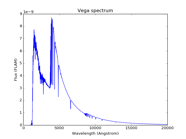
Plot the built-in Vega spectrum, which is used to compute VEGAMAG. This is pre-loaded at start-up for convenience:
>>> from synphot import units
>>> stsyn.Vega.plot(
...     right=20000, flux_unit=units.FLAM,
...     title='Vega spectrum')
Construct a bandpass for HST/ACS camera using WFC1 detector and F555W filter; Then, show all the individual throughput files used in its construction:
>>> bp = stsyn.band('acs,wfc1,f555w')
>>> bp.showfiles()
INFO: #Throughput table names:
/my/local/dir/trds/comp/ota/hst_ota_007_syn.fits
/my/local/dir/trds/comp/acs/acs_wfc_im123_004_syn.fits
/my/local/dir/trds/comp/acs/acs_f555w_wfc_006_syn.fits
/my/local/dir/trds/comp/acs/acs_wfc_ebe_win12f_005_syn.fits
/my/local/dir/trds/comp/acs/acs_wfc_ccd1_mjd_021_syn.fits [...]
Construct a source spectrum from Kurucz 1993 Atlas of Model Atmospheres for a star with blackbody temperature of 5770 Kelvin, at solar metallicity, and log surface gravity of 4.5, renormalized to 20 VEGAMAG in Johnson V filter, using IRAF SYNPHOT syntax:
>>> sp = stsyn.parse_spec(
...     'rn(icat(k93models,5770,0.0,4.5),band(johnson,v),20,vegamag)')
Construct an extinction curve for Milky Way (diffuse) with \(E(B-V)\) of 0.7 mag. Then, apply the extinction to the source spectrum from before:
>>> ext = stsyn.ebmvx('mwavg', 0.7)
>>> sp_ext = sp * ext
Construct an observation using the ACS bandpass and the extincted source
spectrum. (For accurate detector binning, you can pass in the binned wavelength
centers into binset. In this case, the bin centers for that particular
observation mode is stored in bp.binset.) Then, compute the count rate
for HST collecting area:
>>> from synphot import Observation
>>> obs = Observation(sp_ext, bp, binset=bp.binset)
>>> obs.countrate(area=stsyn.config.conf.area)
<Quantity 23.839134880103543 ct / s>
To find out exactly how bp.binset was computed, you can use the following
command, which states that the information for this particular ACS observation
mode in use is stored in wavecats/acs.dat in the stsynphot software
data directory (synphot$, which is named so for backward compatibility
with ASTROLIB PYSYNPHOT):
>>> from stsynphot import wavetable
>>> wavetable.WAVECAT['acs,wfc1,f555w']
'synphot$wavecats/acs.dat'
Calculate thermal background for a HST/WFC3 bandpass for its IR detector using F110W filter:
>>> wfc3 = stsyn.band('wfc3,ir,f110w')
>>> wfc3.thermback()
<Quantity 0.051636304994833425 ct / (pix s)>
Using stsynphot
API
stsynphot.catalog Module
This module handles catalog spectra.
Functions
Empty the catalog grid cache. |
|
|
Extract catalog index (grid parameters). |
|
Extract spectrum from given catalog grid parameters. |
Find valid |
|
|
Visualize the Phoenix catalog index (grid parameters). |
stsynphot.config Module
stsynphot configurable items.
The default configuration heavily depends on STScI TRDS structure
but it can be easily re-configured as the user wishes via
astropy.config.
PYSYN_CDBS must be a defined system environment variable for
directories to be configured properly. It also overwrites
synphot configurable items.
Functions
|
Return current values of select configurable items as a dictionary. |
|
Show the values of select configurable items. |
|
Silently overwrite |
stsynphot.exceptions Module
Custom exceptions for stsynphot to raise.
Classes
Exceptions for language parser. |
|
SPARK AST traversal pruning exception. |
|
Exceptions for catalog problems. |
|
Exceptions to do with graph table traversal. |
|
Unused keyword is not allowed in graph table. |
|
Incomplete observation mode is not allowed in graph table. |
|
Ambiguous observation mode is not allowed in graph table. |
Class Inheritance Diagram
stsynphot.observationmode Module
Module to handle observations based on observation modes.
Functions
Empty the table dictionaries cache. |
Classes
|
Class to handle individual components in |
|
Class to handle thermal components in |
|
Base class to handle an observation that uses the graph and optical component tables, common to both optical and thermal observation modes. |
|
Class to handle an observation that uses the graph and optical component tables. |
|
Class to handle an observation that uses the graph, optical component, and thermal component tables. |
Class Inheritance Diagram
stsynphot.spectrum Module
This module contains spectrum classes specific to STScI formats.
Functions
Empty the reddening laws cache. |
|
|
Interpolate (or extrapolate) throughput spectra in given parameterized FITS table to given parameter value. |
|
Convenience function to create a bandpass with an observation mode string. |
|
Convenience function to create extinction curve for given reddening law and \(E(B-V)\). |
|
Convenience function to load Vega spectrum that is used throughout |
Classes
|
Class to handle bandpass from observation mode. |
Class Inheritance Diagram
stsynphot.stio Module
This module handles stsynphot-specific I/O for:
FITS - See
astropy.io.fitsBasic ASCII - See
astropy.io.ascii
Functions
|
Resolve filename that could be URL or local file. |
|
Convert IRAF filename to regular filename. |
|
Find the filename that appears last in sorted order based on given template. |
|
Read graph table file. |
|
Read component table file (regular or thermal). |
|
Read catalog grid look-up table. |
|
Read wavelength catalog from ASCII file. |
|
Read wavelength table from ASCII file. |
|
Read detector parameters from ASCII file. |
|
Read parameterized (interpolate-able) throughput spectra from FITS table. |
stsynphot.tables Module
This module handles graph and component (optical or thermal) tables.
Classes
|
Class to handle graph table. |
|
Class to handle component table (optical or thermal). |
stsynphot.wavetable Module
Module to handle stsynphot.config.conf.wavecatfile table,
which is used by ETC to select an appropriate wavelength set
for a given observation mode for count rate calculations.
Functions
|
Convenience function to update |
Classes
|
Class to handle |
References
Bessell, M. S. 1983, PASP, 95, 480
Bessell, M. S. & Brett, J. M. 1988, PASP, 100, 1134
Bohlin, R. C., Dickinson, M. E., & Calzetti, D. 2001, AJ, 122, 2118
Bohlin, R. C. & Gilliland, R. L. 2004, AJ, 127, 3508
Brown, M. J. I., et al. 2014, ApJS, 212, 18
Calzetti, D., Kinney, A. L., & Storchi-Bergmann, T. 1994, ApJ, 429, 582
Cohen, M., Wheaton, W. A., & Megeath, S. T. 2003, AJ, 126, 1090
De Marchi, G. et al. 2004, ISR ACS 2004-08: Detector Quantum Efficiency and Photometric Zero Points of the ACS (Baltimore, MD: STScI), http://www.stsci.edu/files/live/sites/www/files/home/hst/instrumentation/acs/documentation/instrument-science-reports-isrs/_documents/isr0408.pdf
Diaz, R. I. 2012, pysynphot/Synphot Throughput Files: Mapping to Instrument Components for ACS, COS, and WFC3, CDBS ISR 2012-01 (Baltimore, MD: STScI)
Earley, J. 1968, An Efficient Context-Free Parsing Algorithm, PhD thesis, Carnegie-Mellon Univ.
Earley, J. 1970, An Efficient Context-Free Parsing Algorithm, CACM, 13(2), 94
Francis, P. J., Hewett, P. C., Foltz, C. B., Chaffee, F. H., Weymann, R. J., & Morris, S. L. 1991, ApJ, 373, 465
Fukugita, M., Ichikawa, T., Gunn, J. E., Doi, M., Shimasaku, K., & Schneider, D. P. 1996, AJ, 111, 1748
Gunn, J. E., Hogg, D., Finkbeiner, D., & Schlegel, D. 2001, Photometry White Paper
Gunn, J. E. & Stryker, L. L. 1983, ApJS, 52, 121
Harris, H., Baum, W., Hunter, D., & Kreidl, T. 1991, AJ, 101, 677
Holberg, J. B. & Bergeron, P. 2006, AJ, 132, 1221
Horne, K. 1988, in New Directions in Spectophotometry: A Meeting Held in Las Vegas, NV, March 28-30, Application of Synthetic Photometry Techniques to Space Telescope Calibration, ed. A. G. Davis Philip, D. S. Hayes, & S. J. Adelman (Schenectady, NY: L. Davis Press), 145
Jacoby, G. H., Hunter, D. A., & Christian, C. A. 1984, ApJS, 56, 257
Johnson, H. L. 1965, ApJ, 141, 923
Kinney, A. L., Calzetti, D., Bohlin, R. C., McQuade, K., Storchi-Bergmann, T., & Schmitt, H. R. 1996, ApJ, 467, 38
Koornneef, J., Bohlin, R., Buser, R., Horne, K., & Turnshek, D. 1986, Highlights Astron., 7, 833
Laidler, V. 2009, TSR 2009-01: Pysynphot Commissioning Report (Baltimore, MD: STScI), https://ssb.stsci.edu/tsr/2009_01/
Laidler, V., et al. 2005, Synphot User’s Guide, Version 5.0 (Baltimore, MD: STScI)
Laidler, V., et al. 2008, Synphot Data User’s Guide, Version 1.2 (Baltimore, MD: STScI)
Landolt, A. U. 1983, AJ, 88, 439
Lim, P. L., Diaz, R. I., & Laidler, V. 2015, PySynphot User’s Guide (Baltimore, MD: STScI), https://pysynphot.readthedocs.io/en/latest/
Lim, P. L., et al. 2016, synphot User’s Guide (Baltimore, MD: STScI), https://synphot.readthedocs.io/en/latest/
Lub, J. & Pel, J. W. 1977, A&A, 54, 137
Lupton, R. H., Gunn, J. E., & Szalay A. S. 1999, AJ, 118, 1406
Maiz Apellaniz, J. 2006, AJ, 131, 1184
Morrissey, P. et al. 2007, ApJS, 173, 682
Oke, J. B. & Gunn, J. E. 1983, ApJ, 266, 713
Pickles, A. J. 1998, PASP, 110, 863
Robitaille, T. P., et al. 2013, A&A, 558, A33
Smith, J. A. et al. 2002, AJ, 123, 2121
Strecker, D. W. et al. 1979, ApJS, 41, 501
van Duinen, R. J., Aalders, J. W. G., Wesselius, P. R., Wildeman, K. J., Wu, C. C., Luinge, W., & Snel, D. 1975, A&A, 39, 159